Feature Engineering With Latitude and Longitude
Leveraging the power in your geospatial data – with code!
Many of today’s most competitive tech markets involve points moving around on a map: ride-hailing services (Uber, Lyft, Grab), micromobility services (Lime, Bird), food delivery services (Delivery Hero, Postsmates, Doordash), and more. Moreover, many services that don’t place customers’ locations at the center of their product use-cases still want to know their customers’ locations so that they can better personalize their experiences based on where they are and what’s going on around them.
What this all means for data scientists is that there’s a lot of latitudes and longitudes floating around our data lakes (pun intended); and buried deep inside just these two variables is a wealth of information!
Creatively and effectively utilizing latitude and longitude can bring immense predictive power to our machine learning applications and added dimensionality to our analytics efforts, helping us data scientists to bring more value to our companies and our customers.
The goal of this article is to give a demonstration of a few feature engineering techniques that use just latitude and longitude, comparing their predictive power on a Miami Home Sale Price Prediction problem. The structure is as follows:
- Miami home sale price prediction problem setup
- Feature engineering experiments
- Raw latitude and longitude
- Spatial density
- Geohash target encoding
- Combination of all features
- Discussion
- Conclusion
Since the focus of this post is on feature-engineering, the model evaluation will be quite straightforward for the sake of brevity and clarity (i.e. no cross-validation and no hyperparameter optimization).
Furthermore, this post will use Polars as a data manipulation library, as opposed to Pandas; if you, dear reader, are unfamiliar with Polars or otherwise find yourself still stuck in Panda-land, feel free to first check out my earlier post, “The 3 Reasons Why I Have Permanently Switched From Pandas To Polars”.
And now, let’s go 🚀
1. Miami Home Sale Price Prediction: Problem Setup
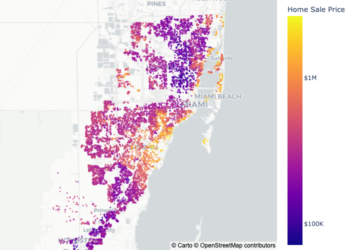
The problem that these different feature engineering techniques will be tested on throughout this post is Home Sale Price Prediction in Miami, coming from a publicly available dataset “Miami Housing 2016” [1]. The only raw features used are "latitude" and "longitude", and they are used to predict the target "price". The feature engineering techniques are compared to one another by way of two different machine learning models: Ridge Regression and XGBoost; here, I use one regression model and one tree-based model to demonstrate the way that these two models respond to the different tecniques considered.
import polars as pl
from xgboost import XGBRegressor
from sklearn.linear_model import Ridge


# Data taken from https://www.openml.org/search?type=data&id=43093
df = (
    pl.scan_csv("../data/miami-housing.csv")
    .with_columns([
        pl.col("SALE_PRC").alias("price"),
        pl.col(["LATITUDE", "LONGITUDE"]).name.to_lowercase()
    ])
    .select(pl.col(["latitude", "longitude", "price"]))
)
Before getting started with any ML prediction, though, it’s necessary to inspect the target variable; after all, monetary variables like “price” and “income” are often log-normally distributed or at least heavily right-skewed, and so it might behoove us to first transform the target variable to log-space:
# Normally, it'd be necessary to take the log of price plus one to account for a log(0)
# error, but there's no way that a house sold for $0 :P
df = df.with_columns(pl.col("price").log10().suffix("_log10"))
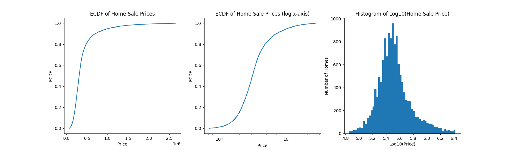
Even after a log transformation, the target is still slightly right-skewed. Nonetheless, it looks sufficient for our use-case.
Now, I just need to add a column to distinguish train and test data, and everything should be good to go:
TRAIN_TEST_SPLIT_FRACTION = 0.8

df = (
    df

    # Shuffle the data to avoid any issues from the data being pre-ordered...
    .sample(fraction=1, shuffle=True)

    # ...then use row numbers as an index for separating train and test.
    .with_row_count(name="row_number")
    .with_columns([
        (pl.col("row_number") < TRAIN_TEST_SPLIT_FRACTION * len(df)).alias("is_train")
    ])
)
And with that, everything is prepared! So without further ado, it’s time to engineer some features 🧑💻
2. Feature Engineering Experiments
2.1. Raw Latitude and Longitude
The first feature engineering technique is… you guessed it – no feature engineering! Latitude and longitude can be quite powerful features on their own, though their behavior as such depends highly on the model being used. In particular, you wouldn’t usually expect latitude or longitude to have a linear relationship with your target variable, unless your target is something earthly in nature, like “temperature” or “humidity”; with this, raw latitude and longitude won’t play so well with linear models like RidgeRegression; they can however already be quite powerful with models based on decision trees like XGBoost:
MODEL_FEATURE_LIST_NAME = "raw_lat_lon"
MODEL_FEATURE_LIST = ["latitude", "longitude"]

X_train = df.filter(pl.col("is_train")).select(MODEL_FEATURE_LIST)
y_train = df.filter(pl.col("is_train")).select(MODEL_TARGET)
X_test = df.filter(~pl.col("is_train")).select(MODEL_FEATURE_LIST)
y_test = df.filter(~pl.col("is_train")).select(MODEL_TARGET).to_numpy()

model_performance_list = []
for model_name, model_class in zip(
    ["xgboost", "ridge regression"],
    [XGBRegressor, Ridge]
):
    model = model_class().fit(X_train, y_train)
    y_predicted = model.predict(X_test)
    model_performance = root_mean_squared_error(y_test, y_predicted)
| ridge regression | xgboost | |
|---|---|---|
| raw_lat_lon | 0.17848 | 0.13420 |
The intuition was correct: XGBoost has a lower root_mean_squared_error than RidgeRegression.
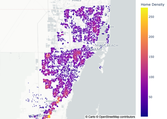
2.2. Spatial Density
Do homes in urban areas sell for higher prices than those in rural areas?
Population density is correlated with many demographic processes, and this is certainly true for rental prices and incomes (e.g. people earn higher salaries in cities than in the countryside). And even though this problem focuses on Miami, where there’s only urban areas and slightly less urban areas, a spatial density feature might still be useful.
One could use many methods for measuring the spatial density around a home: counting the number of other home sales within some radius of each home sale; or computing and sampling from a Kernel Density Estimate over home sale locations; or even pulling third party census data about population density. For this case, I measure spatial density as the number of home sales within some radius of each home, using scipy's cKDtree:
def add_density_feature_columns_to_dataframe(geo_df: pl.DataFrame) -> pl.DataFrame:
    tree = spatial.cKDTree(df.select(["latitude", "longitude"]))
    result = geo_df.with_columns(
        pl.Series(
            "spatial_density",
            tree.query_ball_point(geo_df.select(["latitude", "longitude"]), .005, return_length=True)
        )
    )
    return result


df_w_density = add_density_feature_columns_to_dataframe(df)
And now plugging this new feature into model training…
MODEL_FEATURE_LIST_NAME = "spatial_density"
MODEL_FEATURE_LIST = ["spatial_density"]

X_train = df_w_density.filter(pl.col("is_train")).select(MODEL_FEATURE_LIST)
y_train = df_w_density.filter(pl.col("is_train")).select(MODEL_TARGET)
X_test = df_w_density.filter(~pl.col("is_train")).select(MODEL_FEATURE_LIST)
y_test = df_w_density.filter(~pl.col("is_train")).select(MODEL_TARGET).to_numpy()

model_performance_list = []
for model_name, model_class in zip(
    ["xgboost", "ridge regression"],
    [XGBRegressor, Ridge]
):
    model = model_class().fit(X_train, y_train)
    y_predicted = model.predict(X_test)
    model_performance = root_mean_squared_error(y_test, y_predicted)
| ridge regression | xgboost | |
|---|---|---|
| raw_lat_lon | 0.17848 | 0.13420 |
| spatial_density | 0.12211 | 0.13018 |
Spatial density outperforms raw latitude and longitude for both the regression model and XGBoost; interestingly, the regression model slightly outperforms XGBoost for this feature.
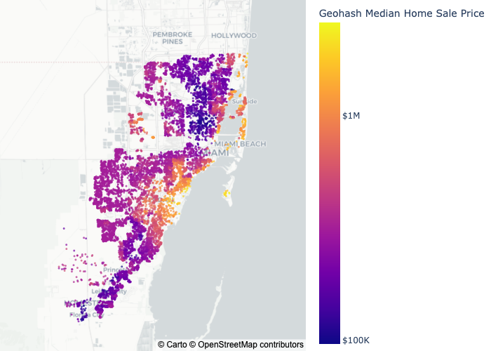
2.3. Geohash Target Encoding
It’s a known fact – some neighborhoods are more expensive than others. So, it’s possible that giving information to the model about each home’s neighborhood (and the sale price that can be expected in that neighborhood) can add predictive power.
But how to do this? Or more immediately, what’s a neighborhood?
A neighborhood can be anything – a zip-code, a street, or in our case, a Geohash. (I recently wrote an article about Geohash and other geospatial indexing tools — how they work, how to use them, and a comparison of Geohash to the two other most popular geospatial indexing tools. Feel free to check it out!)
-> “Geospatial Indexing Explained: A Comparison of Geohash, S2, and H3”
In short, Geohash allows us to convert a latitude-longitude point to a fixed neighborhood, thus giving us homes’ neighborhoods as a categorical variable. And now, equipped with this categorical variable that represents the homes’ neighborhoods, I use target encoding to communicate to the model about the expected price in each of those neighborhoods.
def add_geohash_column_to_df(geo_df: pl.DataFrame) -> pl.DataFrame:
    result = (
        df
        .with_columns(
            df
            .select("latitude", "longitude")
            .map_rows(
                lambda x: geohash2.encode(x[0], x[1], precision=5),
                return_dtype=pl.Utf8
            )
            .rename({"map": "geohash"})
        )
    )
    return result


def add_target_encoding_to_df(
    dataframe: pl.DataFrame,
    categorical_column: str = "geohash"
) -> pl.DataFrame:
    category_target_means = (
        dataframe
        .filter(pl.col("is_train"))  # Only include train data to prevent test data leakage.
        .group_by(categorical_column)
        .agg(
            pl.col(MODEL_TARGET).mean().alias(f"{categorical_column}_{MODEL_TARGET}_mean")
        )
    )
    result = (
        dataframe
        .join(
            category_target_means,
            how="left",
            on=categorical_column
        )
    )
    return result


df_w_geohash = add_geohash_column_to_df(df)
df_w_geohash_target_encoded = add_target_encoding_to_df(df_w_geohash)
Let’s see what the model thinks of my idea:
MODEL_FEATURE_LIST_NAME = "geohash target encoding"
MODEL_FEATURE_LIST = [
    "geohash_price_log10_mean",
]

X_train = df_w_geohash_target_encoded.filter(pl.col("is_train")).select(MODEL_FEATURE_LIST)
y_train = df_w_geohash_target_encoded.filter(pl.col("is_train")).select(MODEL_TARGET)
X_test = df_w_geohash_target_encoded.filter(~pl.col("is_train")).select(MODEL_FEATURE_LIST)
y_test = df_w_geohash_target_encoded.filter(~pl.col("is_train")).select(MODEL_TARGET).to_numpy()

model_performance_list = []
for model_name, model_class in zip(
    ["xgboost", "ridge regression"],
    [XGBRegressor, Ridge]
):
    model = model_class().fit(X_train, y_train)
    y_predicted = model.predict(X_test)
    model_performance = root_mean_squared_error(y_test, y_predicted)
| ridge regression | xgboost | |
|---|---|---|
| raw_lat_lon | 0.17848 | 0.13420 |
| spatial_density | 0.12211 | 0.13018 |
| geohash_target_encoding | 0.12307 | 0.12256 |
Geohash target encoding performs slightly better than spatial density!
2.4: Putting It All Together
Finally, would I really be a data scientist if I didn’t throw all the features together just to see what happens? Let’s do it:
df_w_all_features = add_density_feature_columns_to_dataframe(
    add_target_encoding_to_df(
        add_geohash_column_to_df(df)
    )
)

MODEL_FEATURE_LIST_NAME = "all_features"
MODEL_FEATURE_LIST = [
    "latitude",
    "longitude",
    "spatial_density",
    "geohash_price_log10_mean",
]

X_train = df_w_all_features.filter(pl.col("is_train")).select(MODEL_FEATURE_LIST)
y_train = df_w_all_features.filter(pl.col("is_train")).select(MODEL_TARGET)
X_test = df_w_all_features.filter(~pl.col("is_train")).select(MODEL_FEATURE_LIST)
y_test = df_w_all_features.filter(~pl.col("is_train")).select(MODEL_TARGET).to_numpy()

for model_name, model_class in zip(
    ["xgboost", "ridge regression"],
    [XGBRegressor, Ridge]
):
    model = model_class().fit(X_train, y_train)
    y_predicted = model.predict(X_test)
    model_performance = root_mean_squared_error(y_test, y_predicted)
And the winner is… XGBoost trained on the combination of all features!
| ridge regression | xgboost | |
|---|---|---|
| raw_lat_lon | 0.17848 | 0.13420 |
| spatial_density | 0.12211 | 0.13018 |
| geohash_target_encoding | 0.12307 | 0.12256 |
| all_features | 0.12343 | 0.12037 |
3. Discussion
Of course, as with any data science problem, the fun is only just beginning; there are already many possibilities for improvement:
- Hyperparameter tuning: Is there a more performant choice for search-radius for the spatial density computation? Is there a more performant geohash precision for generating the geohash target-encoding?
- Target encoding: Herein presented was a very basic approach to target-encoding, but can a different approach be taken that improves model generalization, such as Bayesian Target Encoding? Furthermore, could an aggregation function other than just
meanbe used in the target encoding, such asmedian,max, ormin? Evencountwould be interesting as another proxy for spatial density. - Model ensembling: Why just XGBoost and RidgeRegression, and why not a combination of the two? Or, is there even enough data to try training a different model for every distinct Geohash?
And of course, the whole ML approach could be improved to include k-fold cross-validation, or a model or cost function that more richly appreciates the fat-tailed nature of the target variable.
Furthermore, the dataset herein studied was a record of home sales, which is notably distinct from home prices: in the former, one record represents a transaction, whereas in the latter, one record represents an actual home. With that, the spatial density feature herein computed may represent more of a “neighborhood purchasing popularity” than it does urbanness. As with any data science problem, your mileage with these techniques may vary depending on the nature of your data.
4. Conclusion
These are just a few ideas of what can be done when working on machine learning problems with data that contains latitude and longitude; hopefully it gives you some starting points. You can check out the code on my github (link). As always, thank you for reading 🙂 Until next time!
References
[1]: https://www.openml.org/search?type=data&id=43093
Liked what you read? Feel free to reach out on , , , , and .