Geospatial Indexing Explained: A Comparison of Geohash, S2, and H3
Geospatial indexing, or Geocoding, is the process of indexing latitude-longitude pairs to small subdivisions of geographical space, and it is a technique that we data scientists often find ourselves using when faced with geospatial data.
Though the first popular geospatial indexing technique “Geohash” was invented as recently as 2008, indexing latitude-longitude pairs to manageable subdidivisions of space is hardly a new concept. Governments have been breaking up their land into states, provinces, counties, and postal codes for centuries for all sorts of applications, such as taking censuses and aggregating votes for elections.
Rather than using the manual techniques used by governments, we data scientists use modern computational techniques to execute such spatial subdividing, and we do so for our own purposes: analytics, feature-engineering, granular AB testing by geographic subdivision, indexing geospatial databases, and more.
Geospatial indexing is a thoroughly developed area of computer science, and geospatial indexing tools can bring a lot of power and richness to our models and analyses. What makes geospatial indexing techniques further exciting, is that a look under their proverbial hoods reveals eclectic amalgams of other mathematical tools, such as space-filling curves, map projections, tessellations, and more!
This post will explore three of today’s most popular geospatial indexing tools – where they come from, how they work, what makes them different from one another, and how you can get started using them. In chronological order, and from least to greatest complexity, we’ll look at:
- Geohash
- Google S2
- Uber H3
It will conclude by comparing these tools, and recommending when you might want to use one over another.
Before getting started, note that these tools include much functionality beyond basic geospatial indexing: polygon intersection, polygon containment checks, line containment checks, generating cell-coverings of geographical spaces, retrieval of geospatially indexed cells’ neighbors, and more. This post, however, focuses strictly on geospatial indexing functionality.
Geohash
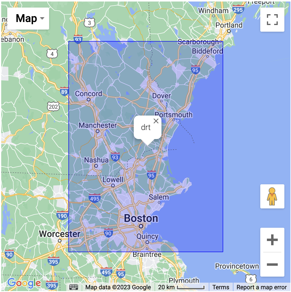
Geohash, invented in 2008 by Gustavo Niemeyer, is the earliest created geospatial indexing tool [1]. It enables its users to map latitude-longitude pairs to Geohash squares of arbitrary user-defined resolution. In Geohash, these squares are uniquely identified by a signature string, such as "drt".
But how are these strings generated?
The Geohash Algorithm
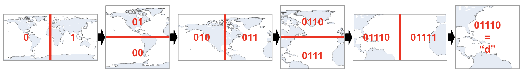
To map a latitude-longitude pair to a geohash is an elegantly simple algorithm:
1. Choose a `geohash-level`, or resolution. For our example, we'll choose `1`.
2. Create an empty binary array `S` of length `geohash-level * 5` (here, length equals `1` times `5`, so `5`).
3. For each geohash level, ask the question `5` times...
    1. Is our point in the left half of the map? If so, append `0` to `S` and reset the map to be just the left half of the map; if our point is in the right half of the map, append `1` to `S` and reset the map to be just the right-half of the map.
    2. Is our point in the bottom half of the map? If so, append `0` to `S` and reset the map to be just the bottom half of the map; if it's in the top half of the map, append `1` to `S` and reset the map to be just the top half of the map.
4. Convert every `5` bits from `S` into a Geohash 32-bit alphanumeric character, and return.
This algorithm can be iteratively repeated arbitrarily many times, all the way down to geohashes that are less than a meter on each side!
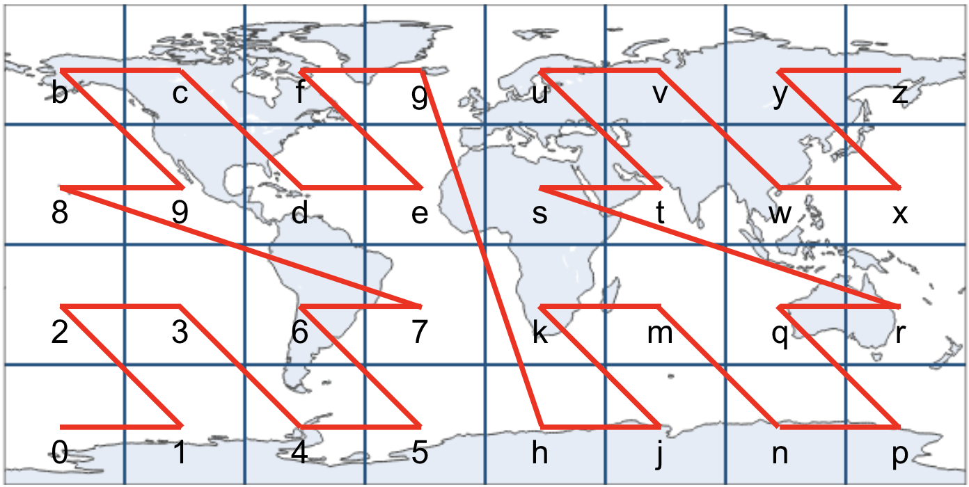
What’s particularly elegant about this algorithm is that, by following this pattern of “left is 0, right is 1; bottom is 0, top is 1”, the alphabetically ordered geohashes trace out a Z-order curve.
What’s a Z-order Curve?
The Z-order curve is a type of space-filling curve, which is designed just for this purpose of mapping multidimensional values (such as latitude-longitude pairs) to one dimensional representations (such as a string) [2].
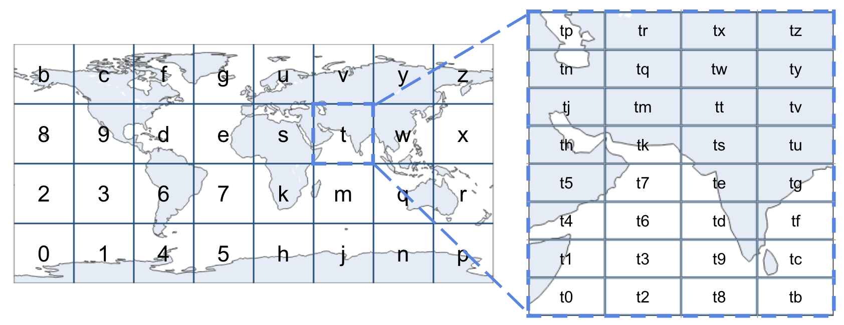
Geohash is quite powerful: it’s simple, fast, and importantly, the geohash strings preserve spatial hierarchy (i.e. if your apartment is in the level 3 geohash "t1a", then it is also in the level 2 geohash "t1", and in the level 1 geohash "t"). However, you might have noticed a few issues with it by now…
Geohash’s Shortcomings
First, while the Z-order curve is convenient, it only weakly preserves latitude-longitude proximity in computed strings; particularly, due to edge effects of the Z-order curve, two locations that are close in physical distance are not guaranteed to be close in their computed geohash strings. Furthermore, due to the “zig-zag” nature of the Z-order curve, the opposite is also true – two locations that are close in their geohash string might not be close in physical distance.
Second, while the equirectangular projection of the globe that is used by Geohash is convenient in its simplicity, it leads to high variability in the size of the geohash squares. Furthermore, this map projection has a discontinuity at both the North and South Poles, so if you live in Antarctica at (-90°, 0°), you will not have a geohash – sorry to disappoint [3]!

Getting Started with Geohash
Being the oldest and most technically straightforward of the three tools discussed in this post, Geohash is also the most ubiquitous. Implementations of Geohash can be found scattered throughout PyPi (e.g. geohashr, geohash-tools, pygeohash-fast), in a Rust crate Rust-Geohash, in a NodeJS library node-geohash, and more. It can also be found as a built-in function in database and data warehouse tools such as PostGIS, AWS Redshift, and GCP Bigquery. I leave experimentation with these tools as an exercise for the reader.
Google S2
First released as open-source on December 5, 2017, S2 was created at Google primarily by Eric Veach [4].
S2, among other things, alleviates the two aforementioned issues with Geohash, and it does so by way of two innovations: (1) it uses a Hilbert curve instead of a Z-order curve to alleviate the problem that string-distance is not representative of physical distance, and (2) it uses an unfolded cube projection instead of Geohash’s equirectangular projection, reducing size differences between cells [5].
The Hilbert Curve
The Hilbert curve is another type of space-filling curve that, rather than using a Z-shaped pattern like the Z-order curve, uses a gentler U-shaped pattern.

By using the Hilbert curve, S2 upholds the promise of locality-sensitive hashing much better than the Z-order curve: though the Hilbert curve possesses the same unfortunate edge effects as the Z-order curve, causing latitude-longitude pairs close in physical distance to not necessarily be close in their S2 Cell ID string distance, latitude-longitude pairs that are close in their S2 Cell ID string distance are much more likely to be close in physical distance.
The S2 Map Projection
The second key innovation from S2 is the use of an unfolded-cube projection of the earth rather than Geohash’s equirectangular projection.
Using such a projection significantly reduces variation between cell sizes because, as you move away from the equator, the distance between two longitude lines increases sinusoidally [5].
Getting Started with S2
Google’s S2 is written in C++, and can be found as a repository in Google’s Github. Enabling the Python interface for this package is possible, however it requires some non-trivial setup. Alternatively, S2 also has ports to Kotlin, Java, and Golang, and there also exists an open-source Python implementation of S2 on Github not written by Google.
Uber H3
Last, and certainly not least, Uber’s H3. The most recently published geospatial indexing tool of these three (published in 2018), H3 has two further key innovations that have made it a very popular tool in data science: (1) the use of hexagons in place of squares, and (2) the use of an icosahedron projection onto Earth [6].

Why Hexagons?
After seeing the elegance of Geohash and S2, you might find yourself asking, “What’s wrong with squares?”. Well, it’s less about what’s wrong with squares, and more about what’s right with hexagons.
The hexagon is the regular polygon with the most sides that still tessellates with itself. And, if you take such a tessellation of only hexagons, the unique property arises that, for any given hexagon in the tessellation, all of its neighbors are equidistant from its center. This property is critically not the same for triangles or squares (the only other two regular polygons that tessellate with themselves), for whom every element of the tessellation has three and two distinct possible distances from its neighbors, respectively [6].
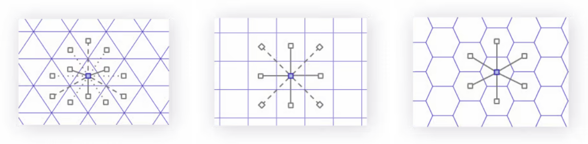
Having this property that all neighbors are equidistant greatly simplifies any calculus or gradient related operations that Uber or H3’s other users might want to perform.
As a brief aside, hexagons are also mother nature’s choice of shape – bees build their hives in hexagons, water crystallizes in hexagons that scale fractally up to beautiful snowflakes, and Saturn has a giant hexagon-shaped storm at its North pole. Put simply, hexagons are the bestagons [7]!
The Icosahedron Projection
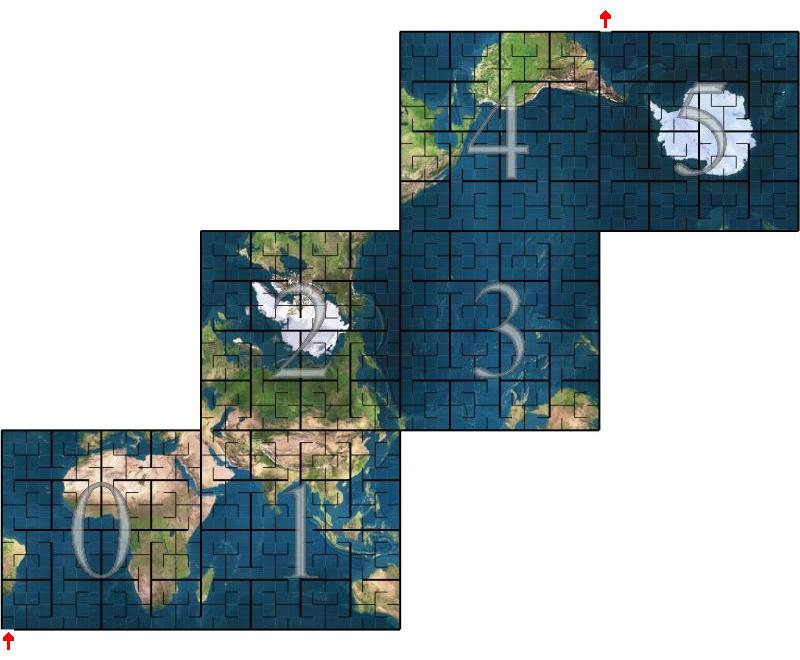
H3’s second innovation is the use of an icosahedron projection (as opposed to Geohash’s equirectangular projection and S2’s unfolded cube).
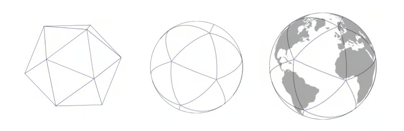
H3 then covers each triangle face of the icosahedron with hexagons, and subdivides hexagons into smaller hexagons from there.
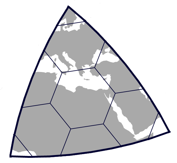
Further note that, the more faces a polyhedron such as the icosahedron has, the closer it approximates a sphere, and thus, the less spatial distortions its projection onto a sphere has. With this, H3’s hexagons have more consistent sizes than S2’s squares, and still more than Geohash’s squares.
H3’s Sacrifices
At this point, you might be wondering – what about a space-filling curve? What about subdividing hexagons into smaller hexagons? Well, there is no such thing as the perfect software architecture – only the right one. And in order to achieve such hexagonal elegance, Uber had to make a few sacrifices.
First: one drawback of hexagons in comparison with squares, is that hexagons don’t quite as cleanly subdivide into other hexagons.
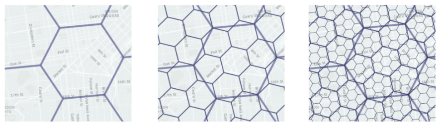
In H3, one hexagon divides into seven other hexagons, in which the resultant subdivided hexagons sit at a slight angle with respect to the larger containing hexagon. The result of this is that the strict spatial hierarchy discussed above regarding Geohash – that if a latitude-longitude point is contained in a cell then it is guaranteed to be contained in that cell’s parent – is not maintained in H3.
Furthermore, by its method of subdividing, while H3 does follow a space-filling curve within each face of the icosahedron, it is not followed globally; furthermore, h3 hexagons’ string identifiers use a bitmap that doesn’t retain the same string-prefix behavior like Geohash [8]. For example, while in Geohash "h356" is the child of "h35", in H3 "862830807ffffff" is the child of "85283083fffffff".
Being the bestagon comes at one final price – while hexagons might tessellate perfectly with themselves on a flat surface, this doesn’t hold on a sphere. To this end, H3’s mapping necessitates that a few pentagons – twelve, to be exact – be placed at the vertices of the icosahedron, just like a football/soccerball. This isn’t too bad, however; the H3 team took care to ensure that all twelve pentagons lay over the oceans [6]!

Getting Started with H3
H3 is actively maintained by Uber. It can be found on Uber’s Github in its primary C implementation; there also exist bindings for Python, R, and many other languages. With this, H3 is far more available than S2, but lacks the cross-platform availability of Geohash. If you want to use H3, it’s quite easy – but you’ll have to stay in Uber’s libraries.
When to Use Which Tool?
The following table summarizes the comparison of Geohash, S2, and H3 across all axes discussed throughout this post:
| Geohash | S2 | H3 | |
|---|---|---|---|
| Release Year | 2008 | 2017 | 2018 |
| Shape of Cells | Square | Square | Hexagon |
| Cells are equidistant from all their neighbors | No | No | Yes |
| Earth Projection | Equirectangular | Unfolded Cube | Icosahedron |
| Size discrepancy between the biggest cell and smallest cell | Large | Medium | Small |
| Space Filling Curve | Z-order Curve | Hilbert Curve | (Not Applicable) |
| Guarantees that cells close in cell-id are close in lat-lon | No | Yes | (Not Applicable) |
| Guarantees that cells close in lat-lon are close in cell-id | No | No | (Not Applicable) |
| Guarantees that if a latitude longitude pair is in a cell, then it is also in that cell’s parent | Yes | Yes | No |
| Cells ids serve as prefixes to the ids of their child cells | Yes | No | No |
| Open-source usability | High | Low | Medium-High |
Rather than answer the question of “when to use which” directly, it might be better to explore a scenario…
Feature Engineering with Latitude and Longitude
Imagine you have a dataset with latitude-longitude pairs as predictors, and some other variable as a target… Geohash, S2, and H3 could all help you, depending on the context!
Are you simply trying to generate a sort of “neighborhood ID” categorical variable by indexing each pair to some geospatial cell? Then yes, any of these tools work.
Or, are you interested in creating some aggregations as features? For example, if you’re trying to predict the lifespan of people and all you have in the training dataset is the people’s latitude-longitude and their lifespan, then it might be useful to compute the feature “what’s the average lifespan of the people who live in this person’s neighborhood?”. Here, “neighorhood” could be Geohash, S2, or H3. However, if you want to compute a feature for “how many people live in this person’s neighborhood?” as a sort of heuristic for population-density of the neighborhood, then it’d be nice for the cells to be the same size, and H3 might be the best choice. If, however, you notice that the latitude-longitude span of the entire dataset is just the island of Manhattan, then in this small area, you can probably use Geohash so that you can enjoy its simplicity without suffering its distortion effects.
Imagine now, however, that you’ve created your features, and you notice that some neighborhoods contain just one or two people (i.e. data points) over your dataset. If that’s the case, then maybe you want to simultaneously use geographic cells of different sizes, in which case, if you use H3, then you might have one person landing up in multiple cells! That wouldn’t be good, so you’d want to choose between Geohash and S2.
And of course, if you happen to be performing some work with ocean-related data, then you might not want to use H3 in order to avoid any pentagon-induced stress.
Conclusion
One charming thing about these three geospatial indexing tools is the historical trend that they trace from innovation to innovation, from Geohash to S2 to H3. As our need for richer features from our systems increase, design complexity increases, and with it, so increase the sacrifices we must make regarding the system’s properties. With this, in the same way that most people today probably prefer using digital calendars for all the multi-device availability and cross-application integrations that they offer, many people likely still opt instead for the analog control and ownership that paper and pen to-do lists and calendars offer.
Anytime we make a choice, whether it’s what to eat for lunch or which geospatial indexing tool to use, we inflect our personalities. And as with any such choice, there is hardly ever a 100% correct answer. What’s your geospatial data problem, and which of these tools might you use to help solve it? Let me know in the comments!
References
[1]: https://en.wikipedia.org/wiki/Geohash
[2]: https://en.wikipedia.org/wiki/Z-order_curve
[3]: https://en.wikipedia.org/wiki/Equirectangular_projection
[4]: https://opensource.googleblog.com/2017/12/announcing-s2-library-geometry-on-sphere.html
[5]: https://s2geometry.io/
[6]: https://www.uber.com/en-DE/blog/h3/
[7]: https://www.youtube.com/watch?v=thOifuHs6eY
[8]: https://h3geo.org/docs/core-library/h3Indexing/
Liked what you read? Feel free to reach out on , , , , and .