Anatomy of a Polars Query: A Syntax Comparison of Polars vs SQL
Transitioning from Pandas to Polars the easy way – by taking a pit stop at SQL.
The secret’s out! Polars is the hottest thing on the block, and everybody wants a slice 😎
I recently wrote a post, “The 3 Reasons I Permanently Switched From Pandas to Polars”, because, well, this is the most common use-case for Polars – as a drop-in replacement for Pandas, for doing single-node data analysis. However, even though this is the most common use-case, transitioning from Pandas to Polars can be a bit strange, given the heavy differences in syntax between the two.
In my earlier blog post, I discussed how Pandas forces its users to perform data queries in an object-oriented programming approach, while Polars enables its users to perform data queries in a data-oriented programming approach, much like SQL. To this end, even though Polars most often serves as a drop-in replacement to Pandas, if you’re trying to learn Polars, comparing it to SQL is likely a much easier starting point than comparing it to Pandas. The objective of this post is to do just that: to compare Polars syntax to SQL syntax as a primer for getting up and running with Polars.
-> “The 3 Reasons Why I Have Permanently Switched From Pandas To Polars”
In this post, I show a syntax comparison of Polars vs SQL, by first establishing a toy dataset, and then demonstrating a Polars-to-SQL syntax comparison of three increasingly complex queries on that dataset.
Note that this blog post uses Google BigQuery as its SQL dialect.
Data Setup
The toy dataset used throughout this post is a table of orders to a restaurant and a table of customers.
orders
| order_date_utc | order_value_usd | customer_id |
|---|---|---|
| 2024-01-02 | 50 | 001 |
| 2024-01-05 | 30 | 002 |
| 2024-01-20 | 44 | 001 |
| 2024-01-22 | 33 | 003 |
| 2024-01-29 | 25 | 002 |
customers
| customer_id | is_premium_customer | name |
|---|---|---|
| 001 | false | Peter Pizza |
| 002 | true | Danny Dumplings |
| 003 | true | Barbara Burrito |
Only four orders in all of January, and only three customers?? This restaurant isn’t doing so well! 😛 Jokes aside, let’s get into some queries 🚀
Query #1: Select, Filter, and Sort
The goal of the first query is to show all orders that were more than $30, sorted by recency, including all columns, but adding another column for the order value in Euros.
In SQL, the query would be like this:
DECLARE usd_to_eur FLOAT64;
SET usd_to_eur = 1.09;

SELECT
    *,
    usd_to_eur * order_value_usd AS order_value_eur
FROM
    orders
WHERE
    order_value_usd > 30
ORDER BY
    order_date_utc DESC;

----------

order_date_utc  order_value_usd  customer_id. order_value_eur
2024-01-22      33.0             003          35.97
2024-01-20      44.0             001          47.96
2024-01-02      50.0             001          54.50
And in Polars, it’d be like this:
import polars as pl

orders = pl.scan_csv("orders.csv")

usd_to_eur = 1.09

(
    orders
    .with_columns([
        pl.col("order_value_usd").mul(usd_to_eur).alias("order_value_eur")
    ])
    .filter(pl.col("order_value_usd") > 30)
    .sort(by=pl.col("order_date_utc"), descending=True)
    .collect()
)

----------

┌────────────────┬─────────────────┬─────────────┬─────────────────┐
│ order_date_utc ┆ order_value_usd ┆ customer_id ┆ order_value_eur │
│ ---            ┆ ---             ┆ ---         ┆ ---             │
│ str            ┆ f64             ┆ str         ┆ f64             │
╞════════════════╪═════════════════╪═════════════╪═════════════════╡
│ 2024-01-22     ┆ 33.0            ┆ 003         ┆ 35.97           │
│ 2024-01-20     ┆ 44.0            ┆ 001         ┆ 47.96           │
│ 2024-01-02     ┆ 50.0            ┆ 001         ┆ 54.5            │
└────────────────┴─────────────────┴─────────────┴─────────────────┘
Referring the Polars query back to the SQL query, it’s easy to see just how similar they are:
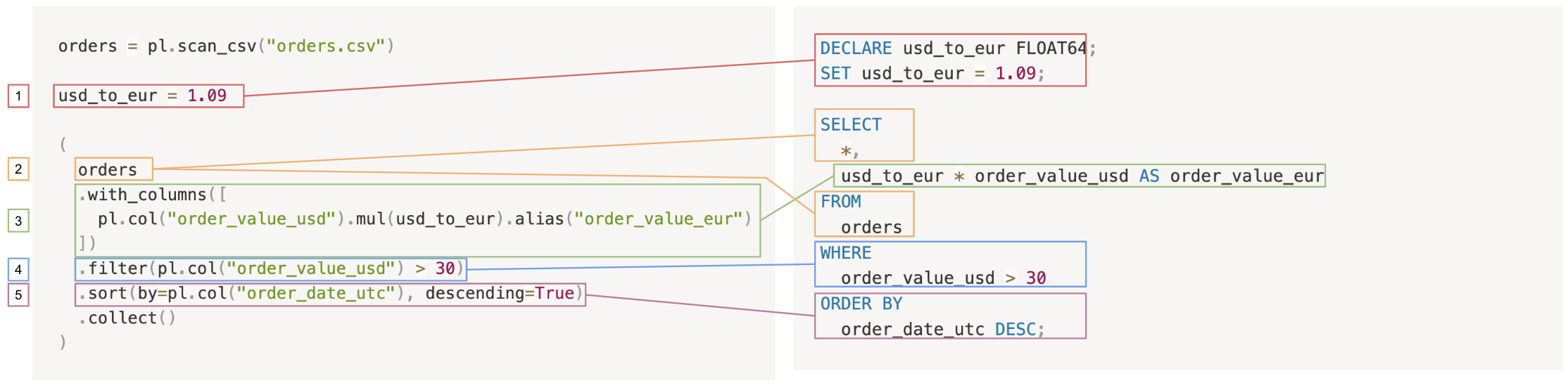
The two queries proceed as follows:
- Create a variable
usd_to_eurfor the currency conversion. - Select all the columns from the orders table: In SQL, it’s
SELECT * FROM orders, but in Polars, theSELECT *is implied by starting from theorderslazyframe. Of course, in Polars, you can also explicitly do this withpl.all(), likeorders.select(pl.all()). - Add a column for the order value in euros: In SQL, this is a simple clause, and in Polars, the new columns must be added to the lazyframe with a
.with_columns()call. - Filter out orders that were less than $40.
- Order by date, in descending order.
Of course, in SQL, you have direct access to the table, while in Polars, you have to start by loading the lazyframe in with pl.scan_csv(). And, if you’re using Polars’s lazy API as is done here, you must also run a .collect() at the end to actually execute the query.
Query #2: Joining and Aggregating
For the next query, we want to answer the question, “How much money has each customer spent in total, by name?”
In SQL, this is:
SELECT
    customers.name,
    SUM(orders.order_value_usd) AS sum_order_value_usd
FROM
    orders
LEFT JOIN
    customers
USING
    (customer_id)
GROUP BY
    customers.name

----------

name             sum_order_value_usd
Barbara Burrito  33.0
Peter Pizza      94.0
Danny Dumplings  55.0
In Polars, it’s:
orders = pl.scan_csv("orders.csv")
customers = pl.scan_csv("customers.csv")

(
    orders
    .join(customers, on="customer_id", how="left")
    .group_by("name")
    .agg(pl.col("order_value_usd").sum().alias("sum_order_value_usd"))
    .collect()
)

----------
┌─────────────────┬─────────────────────┐
│ name            ┆ sum_order_value_usd │
│ ---             ┆ ---                 │
│ str             ┆ f64                 │
╞═════════════════╪═════════════════════╡
│ Barbara Burrito ┆ 33.0                │
│ Peter Pizza     ┆ 94.0                │
│ Danny Dumplings ┆ 55.0                │
└─────────────────┴─────────────────────┘
Comparing the Polars query back to the SQL query:
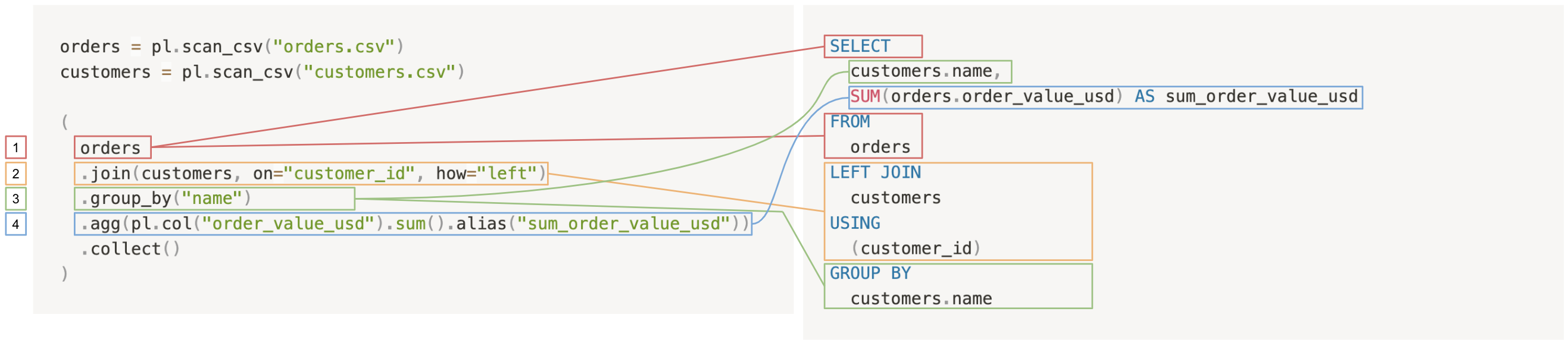
The two queries proceed as follows:
- Select from the orders table: In Polars, this means simply starting from the
orderslazyframe, while in SQL, this requires aSELECT ... FROM orders. - Left join the customers table into the orders table.
- Group by
customer_name: In Polars, grouping by a column implicitly includes that column in the resultant lazyframe, whereas in SQL, even ifcustomers.nameis used in theGROUP BYclause, it must still be explicitly included in theSELECTclause. - Take the sum of all order values for each customer.
Again, if you’re using a pl.LazyFrame rather than a pl.DataFrame, you must still use a .collect() at the end of your query to see the result.
Query #3: CTEs and Window Functions
In this final query, we want to answer the question, “how much money did the restaurant make on the first two premium orders vs the first two non-premium orders?”. Answering this cleanly will require a CTE (Common Table Expression).
WITH orders_w_order_rank_column AS (
    SELECT
    orders.* EXCEPT(customer_id),
    customers.*,
    ROW_NUMBER() OVER
        (PARTITION BY is_premium_customer ORDER BY order_date_utc)
        AS order_rank,
    FROM
        orders
    LEFT JOIN
        customers
    USING
        (customer_id)
)

SELECT
  is_premium_customer,
  SUM(order_value_usd) AS sum_order_value_usd
FROM
  orders_w_order_rank_column
WHERE
  order_rank <= 2
GROUP BY
  is_premium_customer;

----------------------

is_premium_customer  sum_order_value_usd
true                 63.0
false                94.0
And in Polars, it’s:
orders = pl.scan_csv("orders.csv")
customers = pl.scan_csv("customers.csv")

orders_w_order_rank_column = (
    orders
    .join(customers, on="customer_id", how="left")
    .with_columns([
        pl.col("order_date_utc").rank()
        .over(pl.col("is_premium_customer"))
        .alias("order_rank")
    ])
)

(
    orders_w_order_rank_column
    .filter(pl.col("order_rank").le(2))
    .group_by(pl.col("is_premium_customer"))
    .agg(pl.col("order_value_usd").sum().name.prefix("sum_"))
    .collect()
)

----------

┌─────────────────────┬─────────────────────┐
│ is_premium_customer ┆ sum_order_value_usd │
│ ---                 ┆ ---                 │
│ bool                ┆ f64                 │
╞═════════════════════╪═════════════════════╡
│ true                ┆ 63.0                │
│ false               ┆ 94.0                │
└─────────────────────┴─────────────────────┘
Comparing the Polars query back to SQL:
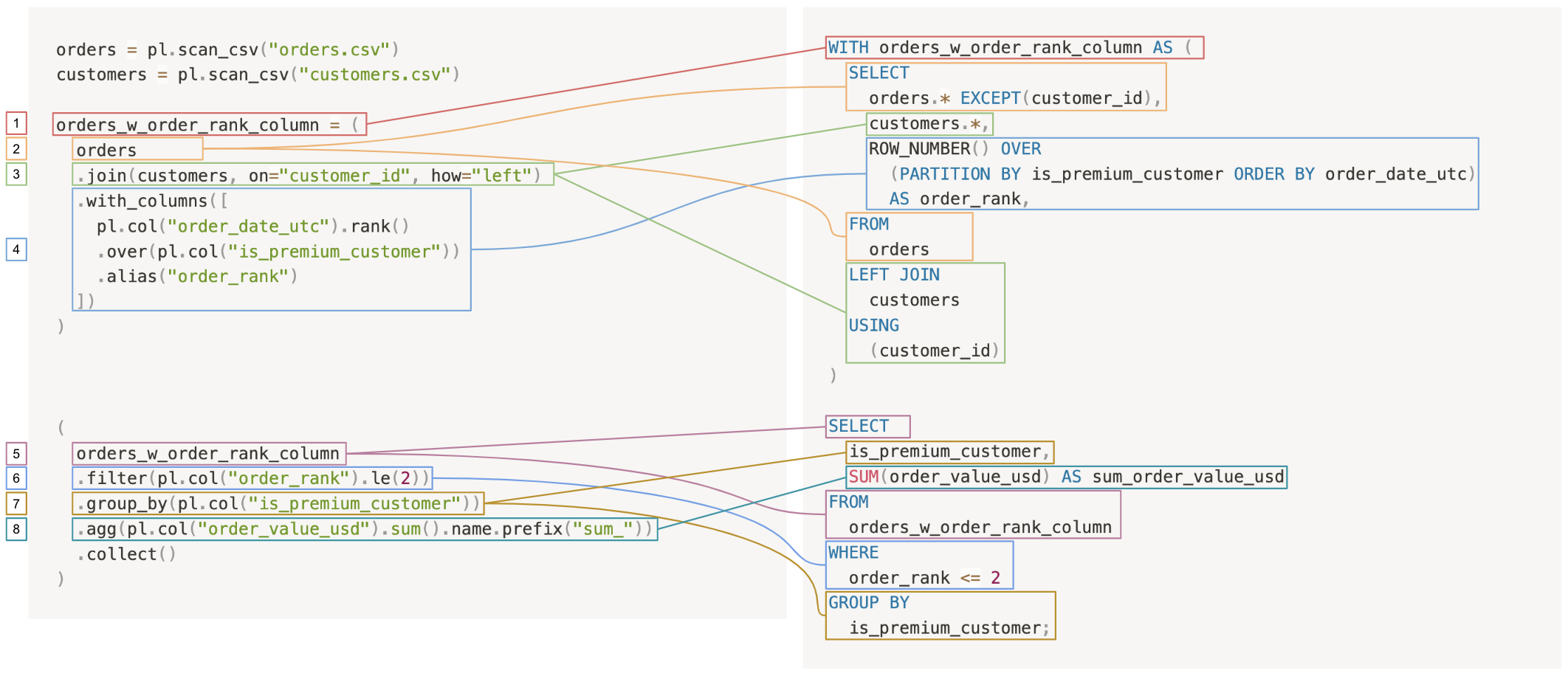 The query breaks down into the following steps:
- Create a CTE of
orders_w_order_rank_column: In Polars, by starting with loading the dataset withpl.scan_csv()statements, creating a CTE is as simple as assigning a query to a new variable,orders_w_order_rank_column. Since it’s operating in lazy mode, Polars doesn’t actually compute this query until it’s used somewhere else. Of course, in SQL, this is done with aWITH orders_w_order_rank_column AS (...)statement. - Select from the orders table.
- Left join the customers table into the orders table.
- Add a column for the
order_rank, partitioned by whether or not the customeris_premium: In Polars, there are a number of tools for operating with window functions (see[pl.Expr.over()](https://docs.pola.rs/py-polars/html/reference/expressions/api/polars.Expr.over.html)). In this case, a convenient call to.rank(), further specifying a partition.over()theis_premiumcolumn. In SQL, this requires aROW_NUMBER() OVER (PARTITION BY ...)clause. - Select from the CTE.
- Keep only the first two orders for each of premium and non-premium orders.
- Group by
is_premium. - For the two groups—
is_premiumandNOT is_premium—take the sum of the total money spent.
And just like that, you’ve got your result!
Conclusion
While Pandas’s ancestry is mixed across Numpy and SQL, Polars’s syntax is more directly inspired by SQL, which becomes readily apparent when comparing Polars to SQL across a few queries. In some cases, Polars is even a bit more concise than SQL!
In the study of foreign languages, it’s generally easier to pick up languages that are closer to your mother tongue; for example, somebody whose native language is Portuguese will likely have an easier time learning Spanish than somebody whose native language is German. And because Polars is more similar to SQL than it is to Pandas, starting to learn Polars by comparing it to SQL can be easier than starting to learn Polars by comparing it to Pandas.
I hope that you’ve found this post useful in either kicking off or continuing on your journey of learning Polars! As always, thank you for reading 🙂 Until next time!